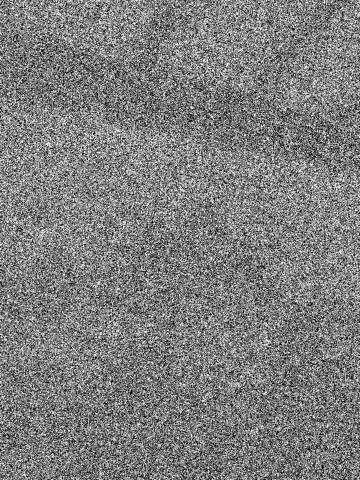
Here you will learn how to fix an image that has been corrupted using gradient descent. Here is the original image and the corrupted version.


We can visualize the process you'll learn like this:

Gradient descent is a simple idea. To minimize a function, it takes the greedy, obvious approach: at each step, it moves a little bit in what currently seems like the best direction. If no direction is improving, then it stops moving.

Imagine the function takes a location on the earth and returns its height above sea level. Now suppose you want to minimize this function, and you start at some point on the earth's surface.

What does gradient descent do? Well, it looks around you a little bit and figures out which direction you can go which will reduce your current height the most. If you were at the top of a hill, you can imagine this would at least work for a while. However, this approach is very unlikely to give you the lowest point on earth! You'll get stuck in a valley at some point where no direction will let you move farther down, and the algorithm will stop.

So, seems like a dumb algorithm, right? Well, kind of magically, gradient descent usually works very well in practice, as we see above.

More formally, gradient descent takes a function and continuously takes a small step away from the direction of the gradient. If you were on a hill, this would correspond to taking a step in the direction of steepest descent.

If our function is convex (basically, there are no "valleys"), then it turns out gradient descent will always find the minimum. However, it often works well enough, even when the function is not convex.

But, enough talk, let's get into the example.

Python has a tool called autograd which, given any function, can find the gradient. We'll use this instead of doing any math ourselves.

Let's say we're given a grayscale image ginkgo.jpg (so, pixel values between 0 and 255) where many of the pixels have been corrupted and replaced with white or black, i.e. value 0 or 255. Let's say 90% of the pixels. At least we know which pixels have been replaced, though (since they have value 0 or 255). Can we approximately recover the original image? Gradient descent says yes.

First let's model this situation in code. We'll also downsample the image to let us deal with a smaller problem. I'll include the packages we'll use here as well.

import autograd.numpy as np
import matplotlib.pyplot as plt
from autograd import grad
from PIL import Image

im = Image.open("ginkgo.jpg").convert('L')
A = np.array(im, dtype=np.float32).T

# downsample
downsample_factor = 4
A = A[0:A.size:downsample_factor, 0:A.size:downsample_factor]

# normalize between 0 and 1
normalized = np.true_divide(A,255)

# get set of correct coordinates
I = np.random.choice(a=[False, True], size=normalized.shape, p=[0.90, 0.1])
# remaining coordinates
R = np.invert(I)
noise = np.random.choice([0,1],normalized.shape)
normalized[R] = noise[R]

Great. Now, normalized is a matrix representing our image with pixel values between 0 and 1. It's already 1/25th of the size (we took the center pixel of every 5x5 block in our downsample section), and then we replaced 90% of the pixels with 0 or 1. Our image now looks like the picture at the top of this guide. We can check it out like this:

# see the image before it is fixed
img = Image.fromarray(normalized*255)
plt.imshow(img)
plt.pause(1)

Now let's define an error function which tries to recover our original image. What we'd like to do is somehow smooth out the image. So, let's incur error whenever two adjacent pixels are different.

def err_func(x):
    score = 0
    for row in x:
        score += np.linalg.norm(np.diff(row)) + np.linalg.norm(np.diff(row[0:row.size:2])) + np.linalg.norm(np.diff(row[1:row.size:2]))
    for row in x.T:
        score += np.linalg.norm(np.diff(row)) + np.linalg.norm(np.diff(row[0:row.size:2])) + np.linalg.norm(np.diff(row[1:row.size:2]))
    print(score)
    return score

You can make this whatever you want, as long as it asks the picture to have some sort of "smooth" behavior. This is smoothing vertically and horizontally on adjacent pixels and pixels that are two apart. Finally, let's implement gradient descent, but keep the pixels we know are right the same. The step size is given by L. In the hill analogy, this is how far you move in the direction of steepest descent every time you take a step. Here we choose to take smaller steps as time passes. Let's also take a look as our image is being fixed.

grad_error = grad(err_func)
for w in range(500):
    # step size
    L = max(1.5/(w+1),0.015)
    grad = grad_error(normalized)
    # zero out gradient of chosen coordinates
    grad[I] = 0
    # do a step
    normalized = normalized - L*grad
    # make sure we stay in bounds
    normalized[normalized < 0] = 0
    normalized[normalized > 1] = 1
    # check out the image
    img = Image.fromarray(normalized*255)
    plt.imshow(img)
    plt.pause(0.01)

And that's it.